Click the Row_num Box and Nest a Match Function

Click the Match_type argument box and type 0. Click INDEX in the Formula bar.

Solved Please Show Steps On The Index And Match Windows Chegg Com

Click the Row_num box and nest a MATCH function.

. Enter the MATCH function in the Row_num field to specify the lookup value. To use MATCH to find an actual question mark or asterisk type first. Type B15 in the Lookup_value box.

Sum of Price is in the VALUES area. Click the Row_num box and nest a MATCH function. INDEXreference row_num column_num area_num In English.

Click the Match_type argument box and type 0. Select cell for the and cells on the sheet for the. Click the Name box drop-down arrow.

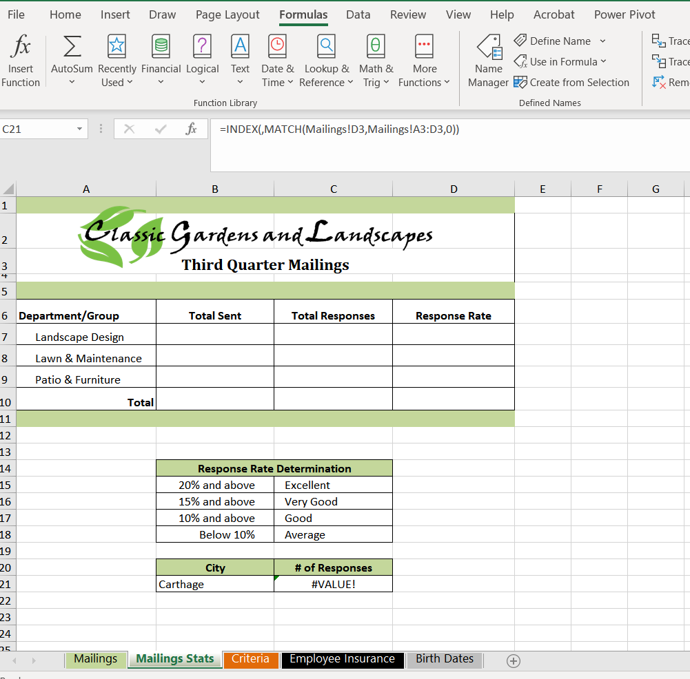
Click the Column_num box and nest a second MATCH function to look up cell D3 on the Mailings sheet in the lookup array A3D3. The index function then displays the value in the column value returned by the match function and in the row specified by the array of cells. Click the Row_num box and nest a MATCH function.

Excel interprets these calculations as a negative cash flow money leaving your account If you would like to show a subtotal of the wholesale price of a number of items of clothing on a PivotTable of data of both men and women. Click INDEX in the Formula bar. The AVERAGE and SUM functions are nested within the IF function.

Click the insert function button fx under the formula toolbar a dialog box will appear type the keyword row in the search for a function box ROW function will appear in select a Function box. Select cell B21 for the Lookup_value and cells A3A28 on the Mailings sheet for the Lookup_array. Gender Item and Price.

Click the Row_num box and nest a MATCH function. Click the Row_num box and nest a MATCH function. Select cell B21 for the Lookup_value and cells A3A28 on the Mailings sheet for the Lookup_array.

You have the following fields. Click the Row_num box and nest a MATCH function. Select cell B21 for the Lookup_value and cells A3A28 on the Mailings sheet for the Lookup_array.

Click the Row_num box and nest a MATCH function. Caution Dont click the formula in the cell. Click cell C21 start an INDEX function and select the first argument list option.

Click the Column_num box. In the Row_num argument box type MATCH. Click cell C21 start an INDEX function and select the first argument list option.

4For the Column_num argument nest a MATCH function using the Function Arguments dialog. Click the Row_num box and nest a MATCH function. Choose or type the Responses range name for the Array argument.

Click the Row_num box and nest a MATCH function. Box and nest a function. Click INDEX in the Formula bar.

Select cell B21 for the Lookup_value and cells A3A28 on the Mailings sheet for the Lookup_array. Click cell C21 start an INDEX function and select the first argument list option. Click the Column_num box and nest a second MATCH function to look up cell D3 on the Mailings sheet in the lookup array A3D3.

Click INDEX in the Formula bar. Double click on the ROW Function. Click the Column_num box and nest a second MATCH function to look up cell D3 on the Mailings sheet in the lookup array A3D3.

Click the Row_num box and nest a MATCH function. Why you should trust IMMENSEWRITERS with your essay Professional Expert Writers. Click the Match_type argument box and type 0.

Select cell B21 for the Lookup_value and cells A3A28 on the Mailings sheet for the Lookup_array. Click INDEX in the Formula bar. The Function Arguments dialog switches over to MATCH.

Select cell B21 for the Lookup_value and cells A3A28 on the Mailings sheet for the Lookup_array. Click the cell in which you want to enter the formula. Click the Match_type argument box and type 0.

You can nest up to 64 levels of functions in a formula. Choose the Responses range for the Array argument. If row_num and column_num dont point to a cell within the array.

Click INDEX in the. Choose or type the Responses range name for the Array argument. INDEXthe range of your table the row number of the table that your data is in the column number of the table that your data is in and if your reference specifies two or more ranges areas then specify which area.

Choose the Responses range for the Array argument. Select cell B21 for the Lookup_value and cells A3A28 on the Mailings sheet for the Lookup_array. Select cell B21 for the Lookup_value and cells A3A28 on the Mailings sheet for the Lookup_array.

The MATCH function should look up the value for the header cell E4 in the range A4E4 with a perfect match. The syntax for the INDEX function is. The nested function returns the value at the intersection of the array column and the value specified in the MATCH function.

Using the mouse go up to the formula bar and click anywhere inside the word MATCH. Select cell B21 for the Lookup_value and cells A3A28 on the Mailings sheet for the Lookup_array. Click the Match_type argument box and type 0.

Click the Match_type argument box and type o. You have to click the formula in the formula bar. A question mark matches any single character and an asterisk matches any sequence of characters eg MATCH Jo110.

Click INDEX in the Formula bar. Click cell C21 start an INDEX function and select the first argument list option. Click the Match_type argument box and type 0.

Gender is in the ROWS area. Click the Row_num box. Click the Match_type argument box and type 0.

Click the Match_type argument box and type 0. To start the formula with the function click Insert Function on the. Click the Match_type argument box and type 0.

Click the Column_num box and nest a second MATCH function to look up cell D3 on the Mailings sheet in the lookup array A3D3. Click the Row_num box and nest a MATCH function. Click the Column_num box and nest a second MATCH function to.

You would start out using the Function Arguments dialog box for INDEX. Choose the Responses range for the Array argument. Click the Row_num box and nest a MATCH function.

Select cell B21 for the Lookup_value and cells A3A28 on the Mailings sheet for the Lookup_array. Select cell B21 for the Lookup_value and cells A3A28 on the Mailings sheet for the Lookup_array. Select cell Click the Row_num box and nest a MATCH function.

Select cell B21 for the Lookup_value and cells A3A28 on the Mailings sheet for the Lookup_array. When you copy this nested function into each successive row it increments the A1 to A2 A3 and so on. Click the Match_type argument box and type 0.

Click the Match_type argument box and type 0 g. Click cell C21 start an INDEX function and select the first argument list option. Click the Row_num MATCH B21 Lookup_value A3A28 Mailings Lookup_array Match_type 0.

If the array is a single column there is no need to add a value to the Column_num field as there is only one column being searched. Click INDEX in the Formula bar. The match function I believe then returns the column letter of where that value was found.

Select MATCH from the Name drop-down list.

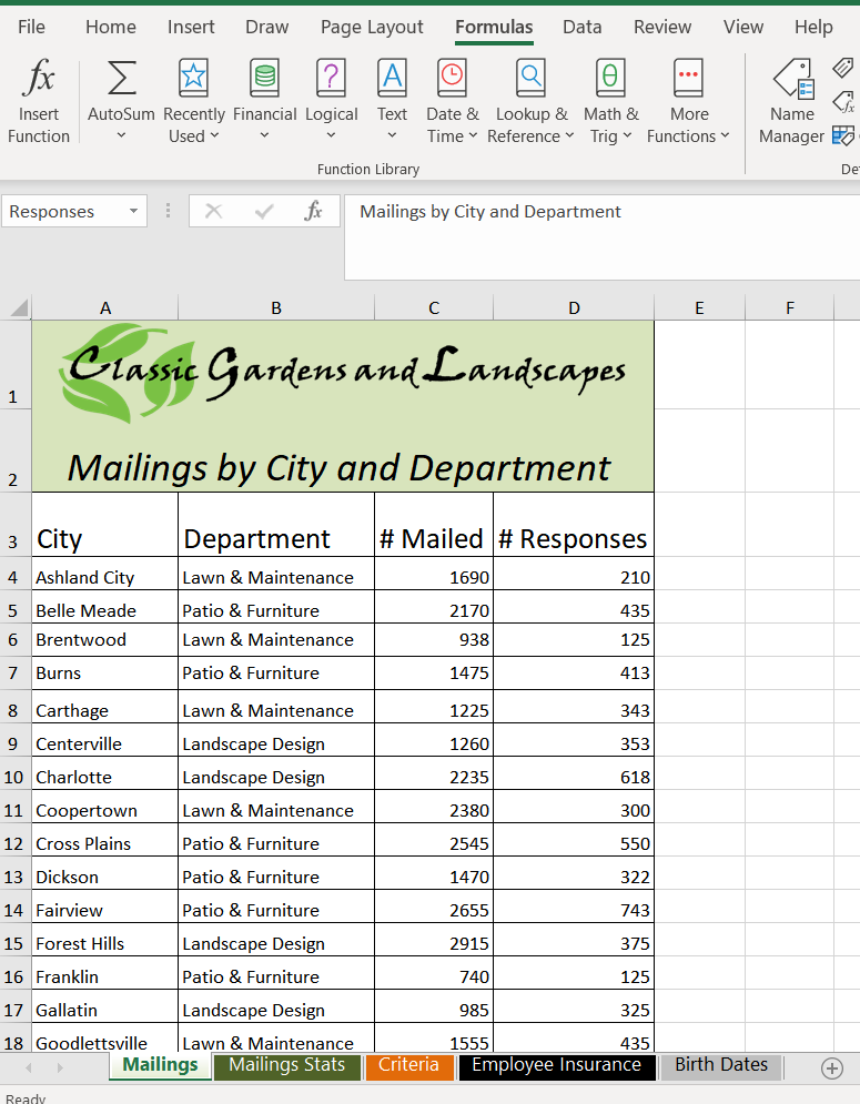
Create A Nested Index And Match Function To Display The Number Of Responses From A City

Create A Nested Index And Match Function To Display The Number Of Responses From A City

Solved Please Show Steps On The Index And Match Windows Chegg Com

Create A Nested Index And Match Function To Display The Number Of Responses From A City